An Introduction to Convolutions and Their Applications in Image Processing
From convolution basics to image classifier algorithms


- What Does Convolution Mean?
- Convolution in Signal Processing
- Convolution in Image Processing
- Building Upwards
- Sources
What Does Convolution Mean?
Definition
Firstly, convolution is a functional operator, meaning it takes two functions as inputs, and outputs a single function. The simplest of functional operations are addition and subtraction. More complex functional operators include things like function composition, where the output of one function becomes the input of the other.
A convolution blends or combines one function with another by shifting or sliding one function overtop of the other, and multiplying the overlapping values at every point of the 'sliding' process. If the functions are discreet, there will be a sum of multiplications, and if the functions are continuous, there will be an integration of multiplications. In this way, the resulting function of a convolution is an expression of how the shape of one input function affects the other input function.
Let's take a look at the convolution of 2 vectors, which can be thought of as discrete functions defined at only 3 points. If A = (1,2,3) and B = (4,5,6), the computation of the convolution would look like this:
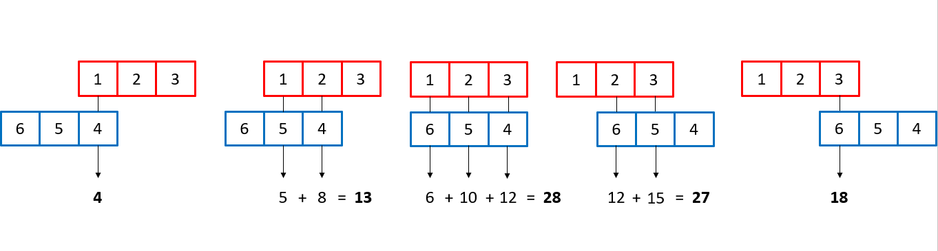
One important thing to note is that vector B (in blue) is flipped. This is to preserve time-causality: basically since 4 is the first value in the vector, it needs to be the first one to multiply with vector A (red) since it 'happens' before values 5 and 6. This step is only necessary for convolutions of functions that are time-dependant. Vector B slides along vector A, and at every point where values overlap, the values are multiplied and then added to each other to give a point-wise result.
The result can be verified using the .convolve method from numpy.
import numpy as np

A = (1,2,3)
B = (4,5,6)

C = np.convolve(A,B)
print(C)
Notation and Properties of Convolution
A convolution operation uses the star (*) operator in a similar fashion to an addition or multiplication symbol. $x(t) * y(t)$ is the convolution of x(t) and y(t).
Convolution is a commutative operation, so $x(t) * y(t) = y(t) * x(t)$. This means that the result of a convolution doesn't depend on which function is sliding overtop of the other, the result will be the same.
Another incredibly powerful and important property of convolution has to do with spectral (Fourier) analysis of functions. Simply put, a convolution of two functions in the time domain is equivalent to a multiplication of functions in the frequency domain, and vice versa. This property is incredibly important in signal processing, image processing, and other areas.
Convolution in Signal Processing
Signal processing is a great intro for convolutions because they are easier to analyze and visualize, as the functions involved generally only require convolution in one dimension, and the function-based nature of convolutions is more apparent.
Let's start with the integral definition of convolution.
$$f(t) * g(t) = \int_{-\infty}^{\infty}f(\tau)\cdot g(t-\tau) d\tau$$
Here, the same idea of one function sliding over another and being multiplied at every point of overlap can still be seen. The main difference between the example shown above and convolutions in signal processing is that signals are usually continuous, so we need to integrate the multiplied functions to collect the overlapping quantities. The functions being convolved are expressed in terms of a dummy variable tau, which is done to differentiate between the variable t, which is now being used to describe the offset that the sliding function has with respect to tau. The preservation of time-causality is seen here again, with g(tau) being flipped across the y-axis.
The links below show an animation of the signal convolution process with different functions. The red and blue shapes are the functions being convolved, and the black shape is the result of their convolution.
Convolution in Image Processing
The Increased Complexity of Working in Multiple Dimensions
In signal processing, signals can be represented as nice, one-dimensional functions quite intuitively. But what about images? It's a lot more difficult to define the frequency, shape, or maximum value of an image, and of course images aren't one-dimensional, so how can the idea of convolutions still be applied?
Higher-dimensional convolutions work upon the same principles we see in signal processing - there are just more steps involved with preparing for convolution, and the convolution process itself. As an example, let's consider the concept of image frequency.
Freqency is just the rate at which some event occurs. For images, the event can be a specific colour. If an image takes many pixels to go from one colour - to other colours - back to the original colour (a smooth gradient), it has a relatively low frequency compared to an image that takes fewer pixels to complete this colour 'cycle', which would have a relatively high frequency.
Similar to the magnitude or value of a function at a point, the magnitude of an image (usually called intensity) is the amount of color present at a specific pixel. For RGB colour images, there are 3 seperate intensity parameters ranging from 0 (no color) to 255 (full color). Because there are multiple parameters, multiple convolutions are needed to analyze color image. For a greyscale image, there is only one intensity parameter, which makes image analysis much simpler.
Finally, we have the problem of dimensionality. Images are 2-dimensional, so, to fully convolve an image, the sliding action that is seen in signal processing must be done along both the width and length of the image.
Kernels (Image Filters)
Just like with signal processing, in image processing we need something to convolve our input with. In this case, this is a convolutional filter called a kernel. A kernel is another matrix that is slid around the image we want to analyze. The values that define the filter depend on what we are trying to accomplish, as will be shown below. Many types of well-known and commonly used kernels exist, such as the Gaussian Blur filter, edge detectors (vertical, horizontal, etc.), and sharpeners. The convolution of these kernels with an image provides the basis for image processing and analysis by altering, or extracting general features from an image.
This animation shows the process of convolving an image (an array of pixel values) with a kernel, which in this case is an edge sharpener. The kernel must be smaller than the image to allow the kernel to slide overtop of the image. For simple image convolutions, 3 x 3 kernels are common. The kernel is centered over a pixel, and the values that overlap with each other are multiplied, and the sum of these multiplications is the output of the convolution (just like with signal processing) for that pixel. This process is repeated for every pixel of the original image.
When the kernel is centered on an edge pixel of the original image, there will be kernel values that do not have image values to multiply with. There are a few ways to deal with this. One way, as shown by the animation, is to extend the edge values. This way, each 'missing edge value' becomes the value of its nearest pixel. Another way is to set all 'missing edge values' to a constant.
Edge Detector Kernels
Sharp edges and lines are incredibly important aspects of an image, as they define broad shapes and forms of the objects within the image. Edge detector kernels, when convolved with an image, highlight and extract these edges. Prewitt edge detectors are an iteration of this type of kernel, shown below.
From the values of the kernels alone, the way the kernels work can begin to be understood. If whatever portion of the image being overlapped by the kernel has no sharp changes in intensity (no edges), the multiplication of the negative row/coloumn added to the positive row/column will result in a very small number, as the negative and positive values cancel each other out. However, if there is an edge present, the multiplication and addition process will result in a large (positive or negative) number at that pixel, denoting that an edge is present.
Below, the process of convolving images with prewitt kernels using Python is shown.
#the skimage library is used to load the filters and perform the convolution operations
#matplotlib is used to display the results

import matplotlib.pyplot as plt
from skimage import filters
from skimage.data import checkerboard, horse
image1 = checkerboard()
image2 = horse()
edge_prewitt_h1 = filters.prewitt_h(image1)
edge_prewitt_v1 = filters.prewitt_v(image1)
edge_prewitt_h2 = filters.prewitt_h(image2)
edge_prewitt_v2 = filters.prewitt_v(image2)

fig, axes = plt.subplots(ncols=3, nrows=2,
                         figsize=(10, 10))

#create sublots
axes[0][0].imshow(image1, cmap=plt.cm.gray)
axes[0][0].set_title('Original Image')

axes[0][1].imshow(edge_prewitt_h1, cmap=plt.cm.gray)
axes[0][1].set_title('Horizontal Edge Detection')

axes[0][2].imshow(edge_prewitt_v1, cmap=plt.cm.gray)
axes[0][2].set_title('Vertical Edge Detection')

axes[1][0].imshow(image2, cmap=plt.cm.gray)
axes[1][0].set_title('Original Image')

axes[1][1].imshow(edge_prewitt_h2, cmap=plt.cm.gray)
axes[1][1].set_title('Horizontal Edge Detection')

axes[1][2].imshow(edge_prewitt_v2, cmap=plt.cm.gray)
axes[1][2].set_title('Vertical Edge Detection')

axes = axes.flatten()
for ax in axes:
    ax.set_axis_off()

plt.tight_layout()
plt.show()

The checkerboard example is very straightforward, as the original image is made up exclusively of vertical and horizontal edges. This makes it a perfect image for an edge detector. However, the image of the horse has more curves, so the edge detectors can't pick up the edges quite as sharply. Since the vast majority of images have more to them than straight, black and white edges, we need to increase to complexity of the filters to keep up.
Building Upwards
Still a Long Way to Go
Simple convolutional kernels like edge-detectors and blur-ers are great, but they are only the first step in creating something as complex and versatile as an image classifier algorithm. Having the ability to classify images based on high-level shapes, intensities, and textures requires more thought and engineering.
A Note on Filter Banks
The most important requirement for creating usable machine-learning algorithms is aquiring enough enough data to train the model on. Although some convolutional image processing algorithms only require one kernel (like the Gaussian Blur kernel shown above), modern machine-learning algorithms use multiple kernels, each extracting different features of an image, to create a larger set of data. When multiple kernels (filters) are used for analysis of the same input, the collection of filters is called a filter bank.
Convolutional Neural Networks vs. Traditional Convolutional Algorithms
Image classifiers and other high-level image processing algorithms present another challenge - it is no longer clear what kernel(s) are needed to solve a particular problem. For example, some images have sharp, vertical edges, so the convolution of a vertical edge detector with the input image extracts a very important feature of the image. Another image may not have any well-defined vertical edges, so the convolution with the same vertical edge detector won't provide much (if any) useful information. The solutions to this problem represent the difference between traditional convolutional image processing algorithms and modern convolutional neural networks (CNNs)...
One simple, traditional solution is to create a large collection of kernels (filter bank). If the kernels are designed such that each one extracts different features from any given image, a subset of the kernel convolution results is bound to contain important information about the image, and thus, analyzing an unknown image with unknown features can be done.
Another solution comes about from the essence of neural networks - using back-propagation and gradient descent, a convolutional neural network learns the values of the kernels it needs itself during the training process based on the features present in the training images. This solution requires no human involvement during the kernel selection and creation process.
CNNs have many clear advantages: the process is independent of a human designer, the creation of the kernels can happen much faster, and with applications involving complex, subtle data, CNNs provide the most accurate results to image processing problems. However, neural networks are computationally expensive, and become 'overkill' for many simpler types of image processing problems. In addition, by removing the designer from the process, it becomes much harder to gain insight about the nature of the data, what issues are still present in the process, and so forth.
Using the Gabor Filter to Create an Image Classifier Manually
An easy, effective way to create a large collection of filters that are sufficiently unique is to use a filter that is defined by a mathematical function, with a number of parameters. This way, to create n filters, we only have to specify n parameters, instead of specifying each value of each m x m kernel. One filter of this type is the Gabor Filter. The Gabor Filter is defined by a Gaussian (defines weights) multiplied by a sinusoid (defines frequencies), with a total of seven parameters.
$$g(x,y,\lambda,\theta,\psi,\sigma,\gamma) = exp\left(-\frac{(xcos(\theta)+ysin(\theta))^2+\gamma^2(-xsin(\theta)+ycos(\theta))^2}{2\sigma^2}\right)cos\left(2\pi\frac{xcos(\theta)+ysin(\theta)}{\lambda}+\psi\right)$$
Each parameter of the function controls some aspect of the filter (orientation, phase, frequency, etc.) and a collection of instances of these filters can be very powerful.
Using a collection of Gabor filters, it becomes possible to create a simple image classifier that can be used for simple tasks. In the linked example below, the Gabor filter method is tested on the MNIST hand-written digit dataset. The same datset is used with a convolutional neural network.
https://github.com/de-fellows/CNN-Gabor-on-MNIST-dataset
The gabor kernel classifier was able to classify hand written digits with 92% accuracy. This is compared to 93% obtained using a neural network on the same dataset. Both algorithms could be altered to improve accuracy somewhat, but in any case it is clear that both methods are powerful and useful for complex imaging tasks, all thanks to the power of convolution.
Sources
Signal Convolution GIFs
Convolution_of_box_signal_with_itself.gif: Brian Amberg derivative work: Tinos, CC BY-SA 3.0 https://creativecommons.org/licenses/by-sa/3.0, via Wikimedia Commons
Convolution_of_spiky_function_with_box.gif: Brian Amberg derivative work: Tinos, CC BY-SA 3.0 https://creativecommons.org/licenses/by-sa/3.0, via Wikimedia Commons
Image Convolution GIF
Michael Plotke, CC BY-SA 3.0 https://creativecommons.org/licenses/by-sa/3.0, via Wikimedia Commons
Gabor Feature Extraction
https://scikit-image.org/docs/stable/auto_examples/features_detection/plot_gabor.html